If you’re working with big Excel spreadsheets, it’s easy to lose track of where you are as you scroll. Your headers might disappear offscreen, and printing can be a hassle when you need your column and row titles visible on each page.
But don’t worry! With a couple of simple Excel tricks, Freeze Panes and Print Titles, you can keep those all-important headings in view—both on your screen and in your printouts. Follow along, and I’ll show you how. Want to see this in action? Check out my video for a step-by-step tutorial!
Excel Freeze Panes vs. Print Titles—What’s the Difference?
Think of Freeze Panes as your on-screen helper, keeping specific rows or columns visible as you scroll. Print Titles, on the other hand, is your go-to for printing, ensuring your headers appear on every printed page. It’s good to know that Freeze Panes and Print Titles don’t “talk” to each other, so you’ll want to know how to use both for different situations.
How to Freeze Rows and Columns

Freeze Panes lets you lock rows or columns in place, making them always visible as you scroll through a large worksheet. Here’s how to keep those row and column labels right where you need them:
How to Freeze (or Lock) the Top Row
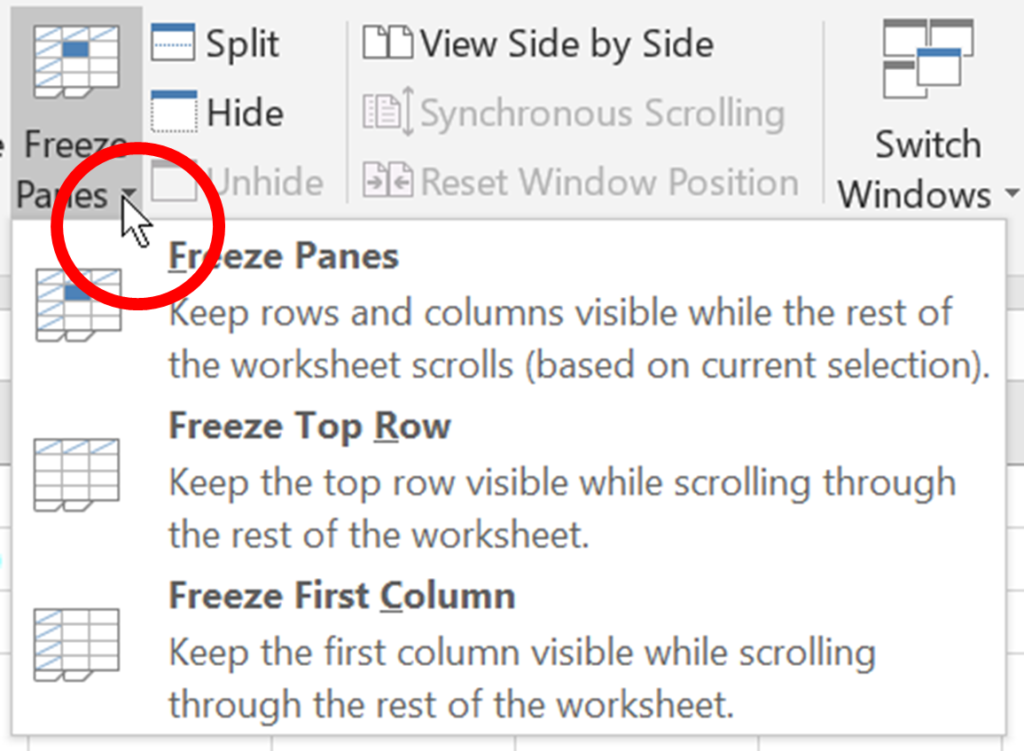
- Go to the View tab Window group, and pick Freeze Panes.
- Next, choose Freeze Top Row. Now, the top row (typically, your header row) remains in place as you scroll down.
How to Freeze (or Lock) the First Column
- Go to the View tab and in the Window group, pick Freeze Panes.
- Next, pick Freeze First Column. Now, the leftmost column (typically, your header column) is anchored even as you scroll sideways.
How to Freeze Both Rows and Columns
Locking or freezing one or more rows and one or more columns onscreen is easier than you might think.
- Simply select the cell below and to the right of the range you want to lock.
For instance, in the example below, the selected cell is D2 to indicate that we want Row 1 and Columns A through C to stay or be frozen on the screen. - Next, in the View tab Window group, click Freeze Panes and Freeze Panes. A thin border displays below the locked rows and to the right of the locked columns. The range will remain in place as you scroll down or to the right.

How to Unlock Rows and Columns
- In the View tab Window group, click Freeze Panes and choose Unfreeze Panes to unlock everything.
Adding Print Titles for Easy Printing
Print Titles are a lifesaver when you need rows or columns to appear on every printed page (whether a PDF or a printout to a physical printer). Here’s how to set it up:
To work with Print Titles in a worksheet:

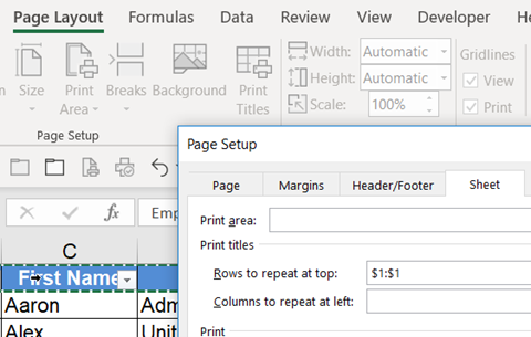
- Choose the Page Layout tab.
- Pick Print Titles.
- Next, from the Sheet tab in Page Setup, choose the options for Rows to repeat at top and/or Columns to repeat at left.
- Click into the worksheet to select one or more rows and/or one or more columns. Excel will fill in the location to repeat on each page, such as $1$1 for Row 1.
- Pick OK to close the Page Setup dialog box.
- Now, press [Ctrl]+P to launch Print Preview.
- Move through the worksheet pages to confirm that the specified row(s) and/or column(s) repeat on every page.
Try these handy tools to make Excel navigation and printing much easier, especially when dealing with large datasets. Give Freeze Panes and Print Titles a try, and you’ll wonder how you ever worked without them!
Discover more Excel tips and tricks, plus download a handout of keyboard shortcuts at TheSoftwarePro.com/Excel.
© Dawn Bjork, MCT, MOSM, CSP®, The Software Pro®
Microsoft Certified Trainer, Productivity Speaker, Certified Speaking Professional
