If you’ve ever needed to summarize the same cell or the same type of data on multiple Excel worksheets, you’ll know this can be quite a tedious process. For instance, to add the values in cell B5 from a series of regional worksheets, the formula might look like this:

=North!B5+South!B5+East!B5+West!B5

Not only is it time-consuming and cumbersome to create these formulas for each total, but the references also are not dynamic. So, if another Excel sheet gets added in the middle, the formula will not update, and your results aren’t correct.

It doesn’t have to be this way! An easier approach to gathering data from multiple Excel sheets to one sheet is with 3D formulas. With Excel 3D references, you can replace this tedious process with a short and flexible formula. Excel 3D formulas are also known as cubed formulas.

To learn more, continue reading or watch my short video on creating 3D formulas in Excel:

Tips for Creating an Excel 3D Formula

A 3D formula refers to the same cell or range in multiple worksheets. For example, the formula =SUM(North:West!C15) sums the data in the C15 cells in the range of North:West worksheets. The key with this is that a 3D formula requires that each worksheet contains the same type of data, such as a worksheet total, in the identical location for each worksheet in the 3D reference. Essentially, an Excel 3D formula “reaches” through the worksheets (the 3rd dimension) to summarize or calculate the data.

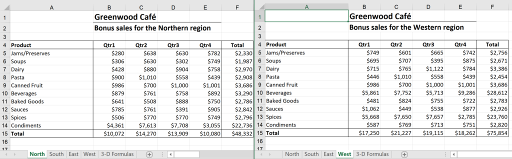
In this example, the same labels, such as Soups, appear in the exact locations in each of these sheets with sales data. Not only do these worksheets contain data for the same products, but we’re tracking the same type of data, in this case, quarterly sales for each of these locations. For instance, data for the 2^nd quarter of the Beverages category is found in cell C10 for each worksheet.

So a consistent layout and data type are key in building a 3D formula. There won’t be as many applications for it, but it still might be a way for you to create links that quickly summarize information with 3D references.

Building an Excel 3D Formula

To insert a 3D reference into a formula:

1. Move to the worksheet where you want to summarize your data.
   If you want to display details from each worksheet, this master or totals worksheet should have the same structure or layout as the worksheets you are referencing.
   If you are only summarizing totals, this worksheet could have a different layout; only the individual worksheets need to share the same structure.
2. Enter the formula until the point where you need a value from another worksheet to complete the formula.
   Although you can use other functions for 3D references, we’ll use the SUM function. For example, =SUM(
3. Click on the first worksheet you want to refer to in the formula. In our example, this is the North worksheet.
4. Select the cell containing the values you want the formula to refer to in the formula.
5. Now, here’s the trick. While pressing [Shift], activate the last worksheet you want to refer to in the formula (in this example, the West worksheet). The selects all of the sheets from the first one to the last one. Notice that they’re all lit up or highlighted.
6. Press [Enter] to complete the formula. Excel will automatically add the close parentheses.

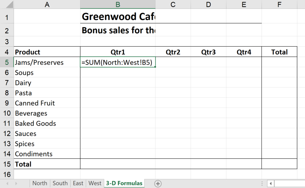
For our example, the formula is:

=SUM(North:West!B5)

The exclamation mark separates the worksheet names from the cell with the sales data.

To complete your calculations:

1. From the master or summary worksheet, select the cell with the formula and copy it down and/or across to other related cells. You can use the fill handle or copy commands. The logic will duplicate to the other cells, so you only need to create the formula once.
2. Add totals and other calculations as needed.

Cautions When Working with 3D Formulas

One of the cautions that we have with this 3D formula approach is to pay attention to managing the worksheets in your workbook. Keep in mind that the three-dimensional reference is a range of worksheets from the FIRST to the LAST worksheet in the range, such as North through West in our example.

• Be careful, then, not to move the worksheet’s position as this may inadvertently move the worksheet and its data outside of the range of the formula. What happens if the South worksheet is moved to the left of the first worksheet, North? We still have a North through West range, but it excludes the South values at this point.
• We can also have the wrong results if we move or add a worksheet that we don’t want to calculate into the range of worksheets.
• And, if you delete a worksheet, it will no longer be a part of the range in the formula, although the calculation may still be correct. However, if you delete the first or last worksheet in a 3D formula range, you’ll need to recreate the formula.

How can you use Microsoft Excel 3D formulas to link and summarize your worksheets?

To be more productive with Microsoft Excel, check out these additional shortcuts, tips, and techniques at TheSoftwarePro.com/Excel.

© Dawn Bjork, MCT, MOSM, CSP®, The Software Pro®
Microsoft Certified Trainer, Productivity Speaker, Certified Speaking Professional